20 years of high-definition simulation in the port industry

More than 20 years of operations, 1,000 projects across 250- plus terminals, over 500 man-years spent on simulation. Sound crazy?

This the story so far for TBA, which is improving the quality of decision-making in ports and terminals. Multi-million projects require a firm foundation of decision-making, which solid models can provide. At the time we started our simulation practice, a large majority of terminals were designed using spreadsheets. It goes without saying that those analyses do not consider the process variations that take place in any container terminal operation. These process variations are a key element, as they are relatively large compared to, for instance, production industry standards.

If we look at the cycle of a quay crane, we see averages in the range of 90 – 120 seconds, with random variations between 60 and 400 seconds. A single cycle can take as long as three times the average. By any standard, that is a high degree of variation. Spreadsheet calculations – also a way of modelling – disregard this randomness, by approximating all parameters by fixed values.

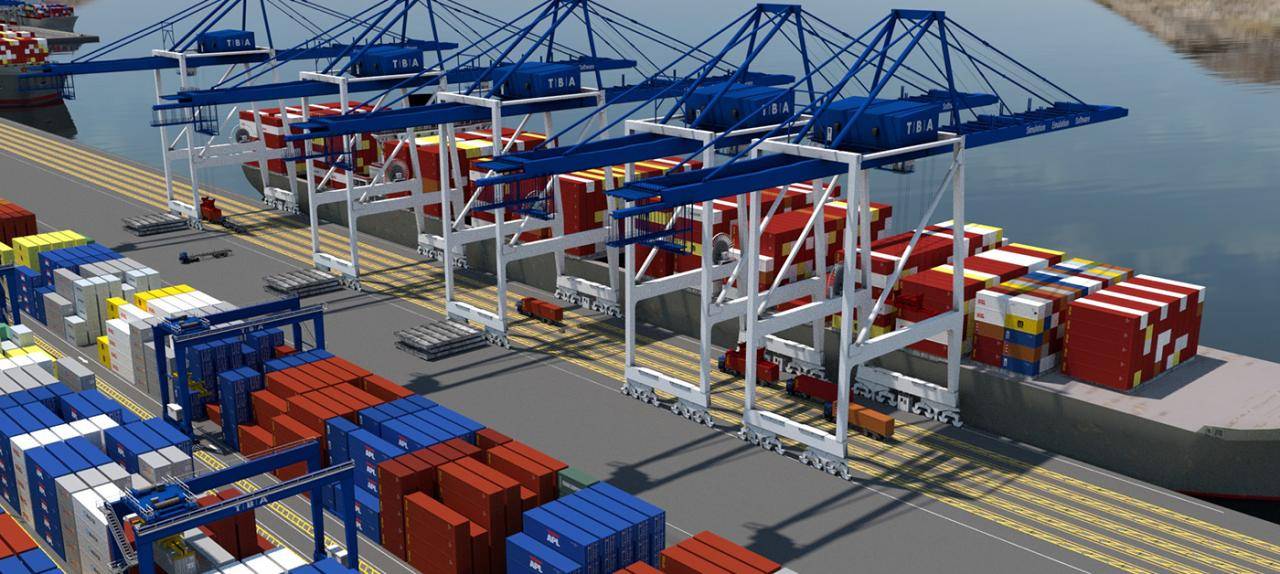
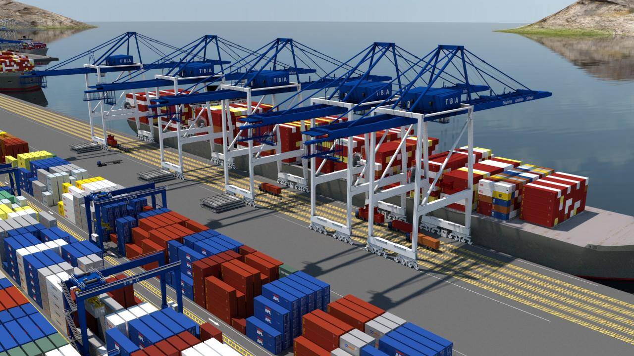
Figure 1: A simple model of a container model, with typical distributions approximating the behaviour of equipment

The impact can be huge. A simple example – which I discuss in my yearly university class, and year after year leads to surprised reactions – involves a terminal with one quay crane, served by two rubber-tyred gantries (RTGs), and a pool of terminal trucks (see Figure 1). In this example, a comparison is made between process behaviour without variations (all process times are constant), and one with the variations shown in Figure 1, but with the same averages.

Figure 2: Results of a simple simulation model comparing results with and without process variation

Then, I ask my students to estimate the difference in realized quay crane productivity, depending on the number of terminal trucks (ITV’s) deployed (the results can be observed in Figure 2). The values in the example including the process variations cannot be calculated. For this, I built a small dynamic simulation model.

The theoretical maximum quay crane productivity is reached with four-and-a-half ITV’s in the situation without process variations, where more than 10 are required. When the stochastic distributions are applied shown in Figure 1. At five ITVs, a difference of more than seven moves per hour can be observed. Intuitively, one can understand what happens – as this can be observed in live container terminal operations as well – sometimes the QC is slow, and a queue of ITVs is built in front of the quay crane (QC).

They lose productivity by waiting for the QC. Similarly, this happens when the RTG is slow: a queue builds there. On the other hand, when a few fast cycles of the QC succeed each other, there quickly is a shortage of ITV’s, as they are still on their way, or still at the RTG. The larger the variation of each sub-process, the greater the loss in productivity (of each of the subsystems).

DECISION-SUPPORT QUESTIONS

Meanwhile, dynamic simulation is widely used in container terminals for a wide range of decisions. To name a few:

• What is the terminal’s berth capacity?
• How many quay cranes are required?
• What is the performance of the yard handling system, dependent on layout, terminal size, fleet size, equipment specifications, etc.?
• How should we optimize the layout to maximize performance?
• What is the impact of the length, width and height of the yard?

Besides these obvious decisions, dynamic simulation finds the answers to more detailed questions such as the required electrical power to feed the terminal, the wear and tear of pavement throughout the terminal, and the impact of more advanced stacking strategies on terminal performance.

To cover the typical questions around terminal design and operational improvement, we have created three base models, which are distinguishable by the time horizon of the experiments:

• Terminal capacity analysis, with a time period covered by an experiment of one year. Herewith, we determine the required berth length, required number of quay cranes, required stack capacity, peak factors for the yard, and water- and landside operation.
• Long-term terminal operational analysis, with a time period covered by an experiment of six weeks. Herewith, we optimize and compare stacking strategies, and see whether especially automated) operations can recover from large peaks.
• Peak operational analysis, with a time period covered by an experiment of 8 to 24 hours. Herewith, we compare handling systems and analyse terminal operations under specific (peak) conditions.

Throughout the years, we have published numerous articles about simulation and presenting simulation results (see the bibliography). Already in 2003, we published a paper based on a comparative analysis of the then-available handling systems for high -density terminals (see Saanen, Van Meel and Verbraeck, 2003).

Recently in PTI, we published an article revisiting this much-discussed topic of ‘the best robotized handling system’ (see Saanen, 2016). As an illustration of the width of the simulation work in the terminal industry, we have included two special cases:

• Congestion free routing of AGV’s
• Design of automated straddle carrier control logic

CONGESTION FREE ROUTING

Around 2004, we evaluated the concept of congestion-free routing for AGVs at an existing AGV terminal. The idea was to pre-plan the execution of a route and only execute it without waiting for other AGVs. We created a model of the terminal that was able to run over 10 times the real-time, including a ‘bit shifting’ algorithm that would determine at what time AGVs should start driving and which route they should take in order to reach their destination without stopping in-between.

While the study showed good results for productivity under optimal conditions, the delay caused by the waiting before departure to get a congestion free route had a negative impact on the overall productivity of the terminal.

The main reason was the accuracy of the real vehicle, the amount of ‘space-time’ needed to reserve for vehicles becomes very large when vehicles do not behave in an optimal way. As soon as one of the vehicles is no longer able to drive according to plan, due to whatever disturbance on the terminal, the concept fails and performance drops.

The alternative of using an inherent deadlock-free routing algorithm combined with the first-come-first-serve principle when driving has congestion problems in specific areas of the terminal, but the concept is much more robust against operational disturbances and it is also easier to mitigate those problems with simple traffic rules.

Until today, this was how TBA routes and controls AGVs at three of the latest terminals at Maasvlakte in Rotterdam. More have suggested the idea of congestion-free routing to us, as an improvement to the relatively simple way of routing AGVs that we apply in our Equipment Control Software.

However, they may seem attractive under optimal circumstances and the process variations of individual vehicles, but also due to the equipment around it, which prove these results too optimistic under live circumstances.

With the incredible increase of computing power and the autonomous vehicle concepts of today, we will have to revisit this topic and perhaps come up with a totally new way of regulating robotized traffic on container terminals.

Figure 3: Comparison of AGV status between congestion free and conventional routing

A-STRAD BEHAVIOUR

Around 2014, Port of Auckland, New Zealand, was investigating future growth potential by changing their manned-straddle -carrier operation to an automated concept (see also Saanen and Gibsen, 2015). In this early stage of automated-straddle development, the industry knew little about how to achieve efficiency from the so-called A-STRADs.

We performed several studies on A-STRAD operations, and are still developing improvements today. A selection of topics that were covered include:

• Implement realistic behaviour of A-STRADs in the simulation model, so that simulation results will be a valid representation of what the real machines are able to do. This process took place in close cooperation with A-STRAD-manufacturer Konecranes - Noell. The A-STRAD movement was implemented in high detail, and time-way diagrams (as shown in picture) were compared between the real and the simulated machine.
• Stack-row management: how to plan moves to, from and through the straddle stack rows, such that A-STRADs can execute their moves quickly, without causing too much hindrance to other A-STRADs, and not get hindered by other A-STRADs. Both the definitions for job dispatching and grounding/storage rules were in coordination with stack-row management.
• A-STRAD routing and claiming: since A-STRADs are quite wide, and some drive actions are relatively slow, it was very important to make good decisions on routing and claiming: which route should an A-STRAD drive such that a number of conflicts between machines remain limited? How to use stack-rows as drive-through-lanes without causing delays to jobs? Where can A-STRADs stand still when waiting for access to specific areas, without blocking other machines?

Figure 4: example of validation chart of A-STRAD behaviour

THE FUTURE OF SIMULATION

Without going at length to where the future goes, we can mention a number of application fields our team is working on. First, besides the application of dynamic modelling for decision-making support, we have an extensive practice in using dynamic models for supporting the testing and tuning mission-critical control software (e.g. TOS).

Besides, we apply the same models for training terminal operators in using this software under ‘near-to-live’ circumstances. The future applications of simulation in the terminal industry will be in real-time parallel simulation and enabling continuous validation of future plans (8-12 hours ahead).

This article has been published in Port Technology International magazine edition 79.